Z-Filters is a technique for listening to what millions of people are talking about.

If a hundred million people were to talk about a hundred million different things, making sense of it would be hopeless, but that’s not the way society operates. The number of things that a million people are talking about in a public forum at any given moment is much, much smaller—thousands, not millions—and by limiting the results to subjects that are newly emerging or newly active, a comprehensive view of what’s new can be seen at approximately the data-flow of the Times Square news ticker.

A video relating to this project can be seen here in Google Drive. It has much the same material as these notes but it shows the program at work.

Depending on how you define ‘subject’, only a few to a few tens of new subjects per minute emerge in the 5000 Tweet/second firehose data stream. It’s worth noting also that newly emerging subjects are usually just a handful of Tweets, which makes sense because after all, they are new.  Major new subjects are typically detected within seconds to tens of seconds. 

This is where Z-Filters comes in. Z-filters detects only new subjects, making it possible to see every subject, which is interesting in itself, but it also becomes possible to watch new subjects develop, because each significant change to a subject makes the subject new again.

A subject that doesn’t evolve into new subjects soon ceases to be new in Z-Filters’ estimation and therefore is no longer seen by the heuristic and fades from view. This is as it should be, because any subject of genuine popular interest tends to be added to continually, keeping it fresh in the eyes of the heuristic. Meaningful subject tend to keep bubbling to the top.

Z-Filters can process the Twitter fire hose in real time, with real time being defined as, with a shorter latency than the time it would take to read and respond to a Tweet, i.e., a few seconds. On a live feed, you could interact with Tweets on a new subject as fast as person could.

The number of Tweets it takes to recognize a subject varies with how fast the burst comes in. A burst of a dozen within an update batch is usually plenty. The same dozen Tweets spread over an hour might not show up at all. Tradeoffs between granularity, latency, and sensitivity are possible by adjusting configuration parameters.

Speed

This kind of performance requires some computational tricks, but the tricks are not as important as carefully defining what it means to listen to millions of voices.

The necessary performance is very hard to achieve if any kind of semantic or NLP processing is allowed in the main pipeline because it’s too much computation. However, if you restrict the view solely to subjects that are new, and leave understanding what the subjects mean as an option for downstream processing, the problem is reduced to human scale and semantic analysis is relatively easy to compute.

This aligns with what happens when a human listens to others talking; in a crowd, you hear that there is a buzz long before you know what people are saying.  The semantic contents are much more diffuse, contradictory, and ambiguous than the simple fact that people are talking about subject X.

Because the heuristic can in principle consume data much faster than X can produce it, fine-grained historical or social research can be performed on large time-spans that would be difficult to handle with analytics that run more slowly that the firehose flow.

The Z-Filters heuristic can achieve a throughput of 50,000 Tweets/second on a low-end desktop or laptop, and can scale almost without limit for historical data that can be processed in large blocks of time by multiple processors.

An AI post-processing semantic analysis processor can be run on the Z-filters output to gain a description of what the subject is about, what entities are concerned, etc. This piece is somewhat slower, but still fast, processing subjects detected by the Z-filters stage with a latency of between one to fifteen seconds. Not quite the near-real-time standard, but close.

Natural Language Processing (NLP), Relative Frequency, and LLM’s

The go-to techniques used for analyzing X, i.e., natural language processing (NLP), relative frequency analysis, and AI using LLM’s, have limitations when applied to the seemingly simple problem of noticing what’s new quickly.  You don’t need to go deeply into specific methods of analysis to see why they can be problematic.

NLP

NLP is strongest at semantic tasks, such as telling you what a piece of text means, or what language something is written in. It also includes an extensive bag of tricks for finding text that is related to subjects that are of a priori interest. With even a vague idea of what one might be listening for, NLP techniques can effectively sniff out the faintest whiff of related Tweets and then work backward and laterally to sharpen their perception.

The problem is, NLP techniques are not as well suited to finding out what’s new, at least not without a large computing infrastructure. One of the biggest reasons is that semantic analysis is computationally heavyweight. For instance, even for the simple task of determining the language of a Tweet, the most effective routine I could find struggled to process more than a hundred Tweets per second, and that’s a much easier task than telling you what a Tweet is about.

More fundamentally, finding out what 5000 Tweets/second are about doesn’t really help with the problem of grouping them into subjects, let alone discovering which of them are new.

Large Language Model (LLM) AI

LLM’s such as GPT are quite good at finding out what a line of text is about, or what a dozen lines of text have in common, etc., but they demand even more computing power than conventional NLP. They tend to take seconds per Tweet, not fractions of a second, and suffer from the same problems that NLP has in that they don’t address grouping Tweets together by subject or deal with the core question of finding out what is new.

Word Relative Frequency

Word-frequency based analysis presents a different set of problems. It can be informative, particularly about big things that are going on, but it tends to be coarse grained.

This is because relative frequency calculations need to operate on the entire set of words currently in use, which is typically in the range of hundreds of thousands to several million.  That’s not a difficult computation for occasional use, but there is a limit to how fast one can perform such global operations.

In our case, we would need to deal with trends in text at a granularity of seconds. With relative frequency techniques, this usually means you not only need to compute relative frequencies at a similar granularity, but you need to keep some kind of history to compare the current frequencies to in order to detect what is changing. This quickly gets to be a lot of computation to perform on the fly every couple of seconds.

You can do it less often, but that transfers the burden onto any clustering phase that groups the Tweets around subjects. Clustering algorithms tend to scale quadratically or even worse, i.e., the work that is required grows out of proportion to the size of whatever batch you are processing.

These Things Do Have a Place

All of these kinds of processing have a place, but that place isn’t in the main flow of a pipeline processing many thousands of Tweets per second.  We’ll see how to apply these techniques more efficiently later on.

What Exactly Is a Subject?

Supreme Court Justice Potter Stewart famously said of obscenity: “I shall not today attempt further to define the kinds of material I understand to be embraced within that shorthand description; and perhaps I could never succeed in intelligibly doing so. But I know it when I see it.”

Subjects are like that—hard to define, but you know them when you see them.  The good news is that even without a good definition, we can do a pretty good job of spotting them computationally based on groupings of a certain category of words.

In principle, two people can talk about a subject without using any of the same words, but that would be unusual.  In practice, clusters of shared words turn out to be a pretty good proxy for the abstraction of subject. This makes sense because the overwhelming majority of words are extremely rarely used (see Zipf’s Law) and it is the more unusual words that make a subject distinctive. A million Tweets on countless subjects include the names Donald Trump or Taylor Swift; it’s the particulars that make a subset of the a new subject.

The great majority of words have frequencies of less than one in hundreds of thousands or even millions. If a handful of words that normally show up once, or perhaps a few times in a day suddenly start popping up together in dozens of the same Tweets within a small time interval, it is unlikely to be a coincidence.

That assertion is easy to support mathematically. If several words that formerly showed up only few times in fifty million Tweets (a day’s worth) suddenly show up together in a dozen Tweets within a minute, a Bayesian perspective tells us that the chance that they are independent events drops close to zero. And to say that their occurrences are not independent is just the backward way of saying the words are being seen together for a reason.

Therefore, for our purposes, we can think of subjects as little rare-word clouds. Counter-intuitively, famous names and highly recognizable words actually matter little when it comes to identifying news. I’m using an older data set where “Bieber” and “Adelle” are so common that they are of little more value than articles like “the” and “a.” They appear in countless Tweets every day.  But when an obscure street name plus the words “egg” and “house” start popping up together in a dozen Tweets, it signifies that something is up long before the name “Bieber”  shows a significant blip in usage.

A Different Way to Look At It

A second key insight is that a word’s frequency isn’t important. A better indicator is that a word’s frequency is increasing rapidly. There is a key difference that is easy to miss: a word’s unusually high relative frequency of usage can persist indefinitely, but frequency can only increase rapidly for a very limited time.

Considering only the leading edge of a surge is powerful because it allows you to shrink the size of the problem. Let’s say we decide that “unusually busy” means that we’ve seen a word more than normally over the last eight hours. There might be thousands of such words. Suppose there were 3000.  There are 480 minutes in eight hours–that’s only 6.25 new exceptionally busy words per minute, or one every 9.6 seconds. To find new subjects, all we have to do is find Tweets that use a cluster of such words from the last few minutes.

This reduces the problem to finding a way to recognize the newly surging words quickly. We don’t even need a way to forget because we can only see new surges.

Objection!

At this point, the reader might reasonably object that it sounds as if we’ve made the problem even harder. With this scheme, we now have to track not only word frequencies but also the rate at which each word frequency is changing over time.

Surprisingly, that is not true. It is possible to detect increases in word frequency many times faster than you can compute the word frequencies themselves.

If you know the background frequencies of words, you can pick out new surges almost as fast as the words fly by. The operative word here is “background.”  You don’t need to know the frequency changes at a fine grain. Every few minutes is often enough, and the computation does not need to take place in the main processing flow or disrupt it in any way.  It is coarse-grained enough that it doesn’t even have to take place on the same machine.

Doing fresh relative frequency calculations every few minutes, even on many millions of words, is not a big deal computationally.

The Trick: Finding the Busy Words Fast

Rapidly computing the set of words that are surging in usage is the interesting part of this process. The rest of the processing involved is very standard—the I/O, JSON parsing, correlations, clustering, etc.—so we won’t talk much about those details here.

The trick to computing the set of words that are newly surging in frequency quickly is doing it without performing relative frequency operations on individual words.

We perform an ongoing background computation of relative word frequency over a sliding window of perhaps a quarter to half an hour of Tweets, but this computation is not in the processing path. Relative frequency is computed over this large window perhaps every five or ten minutes, and the result is used only to refresh a data structure that the main processing pipeline uses to partition the incoming words (tokens) into F frequency-of-use classes.

Detecting the frequency class of each word in the pipeline is a constant-time operation, and very fast; it’s basically just a lookup.

Each of the F frequency classes represents the same amount of word usage, but the most frequently used class might have only a hundred or so words, while the least frequently used class in the data structure might have millions of words.  The very least frequently used class of words are the new ones that have never been assigned a class.

Three-Part Keys

Every word in an incoming Tweet is normalized by case, diacritics, etc., into a token, and each token is mapped to a key.

The key is a set of three different hashes of the token, with each hash taken modulo C, where C is typically in the range of 1,000 to 2,000.  Therefore, the key for a token is three pseudo random numbers in the range [0, C-1].  A mapping of 3pK’s to tokens  and tokens to 3pk’s is maintained globally.

The pipeline processing is very simple. Every incoming word becomes a token,  the frequency class for each token is obtained using the frequency class data structure, then the token’s 3pk is either looked up if it has already been computed, or is computed and added to the lookup table. Finally, the 3pk is put on a queue for the token’s frequency class.  If there are F frequency classes, there are F such queues, and on the other end of each queue is a busy-word processor.

The Busy Word Processors

The busy word processors are simple. Each has three arrays of counters, one for each hash in a 3pk.

Each of the arrays has C counters, i.e., one for each possible 3pK value in the range [0, c-1]. As each 3pk is read in, each of the three values is used to increment the counter that it indexes.

This is the key to reducing the amount of computation. We are not counting or tracking individual words or tokens–only occurrences of each of the three sets of the C possible hash values.

The heuristic deals in batches, which might be in the range of 10,000 to 50,000 Tweets, which would be 100,000 to 500,000 tokens. When an entire batch has been read in, the processor notifies the F frequency processors to stop reading tokens from their queues and process the batch.  

Each processor first performs a Z-score computation on each of the three counter arrays. As the incoming tokens are all in the same frequency class, you expect the counters to mostly have about the same number of hits. There will be a mean count, and most of the counters should not be far above or below that mean value.  The mean counter value should be the total number of tokens from all the Tweets divided by the number of frequency classes divided by C. 

If you’ve forgotten your statistics, the Z-score of each counter position is the mathematical description of how surprising each count’s deviation from this mean is statistically. 

If the incoming data were normally distributed, as it would be if the Tweets being processed were the same Tweets that were used to build the frequency class data structures, you’d have very orderly set of Z-scores in a bell curve around the mean of 0. (The mean Z score is always 0.) 

With normally distributed data, about two-thirds of the Z-scores would be between -1.0 and 1.0, so a Z score in that range is completely unsurprising. You’d see a Z score greater than about 3.1 only about one time in a thousand, so a Z of 3.1 is a little surprising. A Z greater than 4.0 would occur only once in 31,574 events, so 4+ would be very surprising.

The trick is, while most of the words will be normally distributed. We are expecting a few words in each frequency class to be freakishly busy, i.e., to completely fail to conform to the background expectation. These are the words that characterize a burst of Tweets on some subject, and detecting these anomalies is the point of the exercise. 

These index counts for these few abnormally frequently used words will overlay the nice, normal distributions with the exceptionally high counts for those tokens. Thus, a few counters will have extraordinarily high Z-scores that would almost never be reached if the words had their normal background random frequency. The busy words might produce a sprinkling of Z-scores that are in the double digits–something that would never in a million years happen in normally distributed data.   The index of any counter with a Z-score above four is probably from one or more busy words.

Purists may object that strictly speaking, Z-scores are for continuous data, not integer counts, and they assume a normal distribution, which we explicitly do not have. True, but those facts notwithstanding, this general technique for detecting anomalies is common. Incidentally, you can confirm that the underlying data is fairly normal because you can see in the logs that the left hand side of the Z-distribution tends to be very ordinary, with values rarely going lower than -3.0.  Only the right side, where the exceptionally common events register, will show the spiking Z-scores.

The spikes are the signature of the busy words.

Identifying The Words

The next problem is turning the spikes back into tokens.

For each busy word processor, we select the indexes with the freakishly high Z-scores into three sets (which are each much smaller than C), one for each counter array. The counter indexes are values from the 3pk’s. 

Therefore, the 3pk’s of those tokens are in there somewhere, and if we can find them, we can recover the corresponding tokens.  The problem is, which triples of indexes do we use to construct the keys? A spike in one set could be matched up with any spike in each of the other sets.  

We solve this problem by creating all the possible 3pK’s that can be created from the three sets of indices, i.e., we take the Cartesian product of the three sets. 

All the keys we want are in the Cartesian product, but so are a much larger number of spurious keys. This is because the cardinality of the Cartesian product is the product of the number of spikes in each of the three sets, but the number of tokens that produced them is approximately equal to the number of spikes in each set.

Fortunately, the ones we want will all have mappings that exist in the 3pk to token map while very few of the others will. This is why we use a large C value. A few of the 3pk’s we have generated might, by chance, map to some random token that happens to exist even though the token wasn’t never seen, but it won’t be many, and as we will see, it doesn’t matter much if a few do.

The effect of this is that without counting any actual words, we have identified all the freakishly busy words in the frequency class, and done it in an amount of time that is tiny compared to the work of just reading in the Tweets (around 1%.)

Why won’t there be many false triples? The size of C is a configuration parameter, but the best values will in the 1000 to 2000 range. C cubed is the size of the key space, so if C=1000, there are a billion possible 3pk’s. If C=2000, there are eight billion possible keys.  By only keeping mappings for 3pk’s that have been seen in the last several million tokens, the number of distinct 3pk’s that exist at any one time is ordinarily in the hundreds of thousands. Therefore, the chance of a random 3pk mapping to an existing token would be well under one in a thousand.

The Birthday Paradox tells us that the chance of some spurious token colliding with a real word is much greater, but it actually doesn’t matter much. This is because most words are very rare, which means the chance that a given spurious busy word will occur in a current Tweet is quite small, and the chance that it will occur in a current Tweet with other words that have been correctly identified as busy is vastly smaller still.

What Are The Criteria for Choosing C?

How do you choose the value of C? It’s a balance.

Processing small batches of Tweets keeps the latency low and the granularity of the analysis fine. It also minimizes the number of subjects that the non-linear clustering operation works on.

However, Z-scores are more reliable with a bigger batch size because the larger the number of tokens, the smaller is the variance.

C should be big enough to produce a large enough key space to hold the rate of collisions down, which argues for a large C, but a large C requires bigger batches to keep the variance down and the accuracy high. (You want big enough value in each counter.)

Quantifying exactly how big is optimal is an open question, but C in the range of 1000 to 2000 seems to strike a good balance. This range keeps the size of the key space in the low billions while achieving a reasonable balance of batch size and Z-score quality.

Identifying  the Subjects and Clumping the Tweets

Processing intervals are typically a few seconds of the firehose, i.e., a few tens of thousands of Tweets, which can be stored in-memory in just a few megabytes. Therefore you can easily keep the most recent several intervals of Tweets in memory for fast analysis.

With the busy words for the current interval in hand:

• All Tweets for the interval that do not contain a minimum number of the identified busy words are set aside.
• Using a standard graph clustering algorithm, the remaining Tweets are clustered into sets based on the subsets of the current busy words they use.  These clusters are the subjects.
• A medoid is computed for each set–this is the most lexically typical Tweet in the set.
• Optionally, Tweets from the preceding interval or intervals can also be scanned for words that had not yet made the grade but subsequently did.  This is valuable for finding the origin of a subject because the subject may exists as only a single Tweet, or a handful of Tweets for multiple cycles before it can be identified statistically.

Tweet clumps may have overlapping sets of busy words because what a person would judge to be “a subject” can be several overlapping subjects as seen by the heuristics. What one often finds is that the overlapping clusterings show different aspects an ongoing conversation.

In practice, this works very well. Over the course of a football game or other mass event, the high points can easily be recognized in the Twitter stream as new words get sprinkled in among the busy words that originally identified the subject.

A Major Event

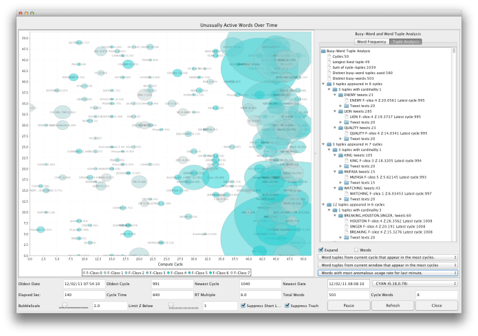
One notable example of subject-discovery in the two-week sample data set relates to the death of the singer Whitney Houston, which produced the biggest surge of Tweets that had ever been seen. A video of the GUI running at this time can be seen here. The algorithm picked up on the event within about a dozen tweets—barely time for re-Tweeting to have gotten under way.

Significantly, neither “Whitney” nor “Houston” was among the early words that stimulated notice of the Tweet subject. The two names are moderately common words that normally appeared (until then) a few dozen times a day, together and/or separately. The words that first surged beyond the possibility of random chance were the names of her publicist, who was one of the first to Tweet the news. Other early subjects included “bath” and similar words associated with the early rumors. This is the expected behavior because famous names appear all the time, so it takes a large number of Tweets to constitute an unambiguous surge. Surges of usage of unusual names and words are much more likely to signify something new and interesting than are changes in the frequency of more common names and words, if only because it takes so many more usages to move the needle with a common name.

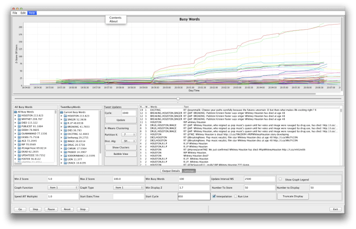The two illustrations show different views of this sad but interesting moment in Twitter history. Seconds earlier, the new talk was (and had been for many minutes) about a Lion King special, a South American band, and a number of other ephemeral subjects. You can see in the screen shot just above the minute when news of the singer’s death explodes. The graph covers about six minutes of the feed.

Bubbles: The bubble view (at the beginning of this article) shows 140 seconds of busy words.

• The lava-lamp on the right represents many words relating to Whitney Houston but also words from other subjects that have not yet disappeared.
• The intensity of color indicates a word’s frequency class.
• The position from right to left indicates how long it has been since a given word was detected surging. All the way on the right indicates that a word is surging in the latest interval. If a word somewhere to the left suddenly surges again, it will pop back over to the far right.
• The size of the bubble indicates the degree of abnormality of usage adjusted for frequency class. (seven frequency classes were used in this run).
• The text output shows sample tweets for each subject ordered by how long the subject has been surging (as opposed to merely existing.) Tweets about the singer, though overwhelmingly common, are not yet at the top in this display because the event just happened, so they have only been surging at most about three minutes.

Main Screen: This view shows an elapsed time view of the last six minutes at about the same time.  The moment where the lines erupt is only about six seconds after the first Tweets about the singer’s death. (This is not evident in the output, but was verified by a utility that scans the Tweet stream by brute force.)

• The X axis represents time, covering about six minutes.
• The Y axis represents the nominal Z-score
• The lines represent the surging of individual words over time in terms of the nominal Z score. This is not a word’s frequency of usage, but the improbability of the first derivative of that frequency occurring by random chance. Interpret it as the steepness of increase.

The earliest Tweets about the event showed the significant words being Foster, publicist, and Kristin because even a dozen or so instances of these words within a few seconds represents a huge increase in usage.

Adding AI with Ollama

Z-Filters does a great job of finding subjects.  It’s natural next step to hook it up to an LLM for semantic analysis of the subjects. In this way millions of inbound Tweets can be converted to a steady drip of human-language descriptions of new things people are talking about. It’s easy because the data volume is reduced by a factor of many thousands.

To this end, a feeder program monitors the Z-Filters output and inserts the subject-clusters into a Postgres database. There are tables for each batch and its metadata, cluster and cluster metadata, subject Tweets from that batch along with the Tweet metadata, and the relevant busy words.   Database inserts add negligible processing time compared to the batching interval.

The second feeder takes the new cluster/subjects database rows as they come in to Postgres. The feeder assembles each cluster of Tweets into a prompt, and passes it to an Ollama LLM via an HTTP POST.

Ollama’s analysis response is inserted into the SQL database, where it is available to be joined with both the Z-filters data and other AI data.

On a desktop platform, the main contributor to latency is the Ollama call, which takes about fifteen seconds per batch with the Ollama LLM running on an ordinary laptop. Fifteen seconds per batch is somewhat slower than the full firehose rate, but that’s for serial computation. You could run Ollama on multiple machines to get as much throughput as required. 

Fifteen seconds processing time is also a hit to latency, but it could be pushed to the one to two second range with proper hardware (a high end graphics board.)

What’s It Good For?

One of the weaknesses of X/Twitter has always been that it punts the problem of finding out what is going on to the users. You either have to know by some other means, e.g. conventional media, or look for hashtags that someone has explicitly applied, or participate with others who will send things your way.

Simple though it is, the Z-filters approach makes it possible to discover what is happening globally across the totality of X at a fine grain, opening a more broadcast-like mode of communication within Twitter. Being able to watch the new topics scroll by allows users to drop in on anything that looks interesting as it happens.

Speed is just as important for historical analysis as it is for real time. It isn’t practical to examine years of data if it takes years to do it. Nor is it practical for academics to do it if it requires a huge computing infrastructure. Consuming data at 10x the realtime rate using a minimal platform could make a big difference in what is practical. Moreover, one can apply separate instances to process as many time slices as needed to achieve almost any desired speed.

Historical processing was actually the original motivation for the project. The ability to analyze the flow of ideas in the crowd during complex events such as the Arab Spring uprisings, BLM, or the spread and nature of conspiracy theories might be another.