I want my big-data applications to run as fast as possible.  So why do the engineers who designed Hadoop specify “commodity hardware” for Hadoop clusters?  Why go out of your way to tell people to run on mediocre machines?

Thanks to Moore’s Law and the relentless evolution of programming technologies, the capacity of relational databases has grown literally exponentially since they first came out at the end of 1970’s. But as early at the 2000’s, it had become clear that the data volumes generated by millions of Internet users would dwarf even that extraordinary growth curve.

Indexing the World Wide Web was one of the core problems—by 2005, Yahoo!, which at the time had the world’s most powerful search engine, was already indexing 20 billion Web pages. (Google, the 2015 champ, claims to index an incredible 30 trillion pages—petabytes for the URL’s alone!) Neither relational technology nor the batch processing technologies of the day showed much promise of being able to deal with a rising flood of that magnitude.

Two famous papers from Google in 2004 pointed to solutions:

• BigTable: A Distributed Storage System for Structured Data
• MapReduce: Simplified Data Processing on Large Clusters.

The first of these formed the root of HBase (as well as several other NoSQL databases) and the second, starting in 2005, was developed at Yahoo! into Hadoop/MapReduce. The purpose of Hadoop was to allow batch processing at almost unlimited scale through the application of three principles:

• Massive parallelism
• A share-nothing architecture
• Moving the code to the data (rather than the other way around)

The unspoken principle was affordability. Processing the anticipated data volumes at a price-per-gigabyte that was anything like the prevailing cost for high-end processing solutions would have been prohibitively expensive. In this respect too, Hadoop was a smashing success; at this writing, Hadoop storage costs as little as 1% of the equivalent amount of space on a compute appliance.

Reliability

Computers and disks are remarkably reliable. Disk drives have a mean time before failure (MTBF) of between one and two centuries and CPU MTBF’s, though shorter, are still typically several decades—an order of magnitude longer than the time-to-obsolescence for a chip. A fresh-faced intern plugging in a server today could expect to be retired before that server died a natural death.

The MTBF’s of typical SATA and SAS disk drives are around 130 years and 180 years respectively, which sounds pretty good, but even a moderately large Hadoop cluster might have 1000 nodes, each with as many as 24 such drives. That’s 24,000 disk drives. If we make the simplifying assumption that drives fail at random, and we’re using SATA drives, that implies a failed drive every couple of days. Add in failures among the 2000 CPU’s, blown disk controllers and network cards and other assorted faults, and hardware failure becomes a daily occurrence. And remember, a thousand machines is just pretty big—there are Hadoop clusters out there that are as much five times that size.

High-end databases and data appliances often approach the problem of hardware failure by using RAID drives and other fancy hardware to reduce the possibility of data loss. This approach works well at modest scale, but it breaks down when you have thousands of machines. Even if you could bump the MTBF up by a factor of 10X it wouldn’t solve the problem—instead of failing a few times a day, the cluster would fail once a day, or every couple of days.

Hadoop takes a different approach. Instead of avoiding failure, the Hadoop designers assume that hardware failure will be routine. Therefore, HDFS duplicates data three times, with each copy on a different machine, including copies on two different racks if possible. If a disk, a machine, or a rack fails, the HDFS NameNode notices quickly and starts replacing the missing data blocks from the replicas to a sound drive or machine. If a hardware failure causes a component process of a job to die, it doesn’t derail the entire job. Instead, the MR framework detects the failure quickly and runs that one chunk again elsewhere.

Because hardware failure is inevitable and planned for, with a Hadoop cluster, the frequency of failure, within reason, becomes a minor concern because even the best disks will fail too often to pretend that storage is “reliable.”

It takes a major disaster to lose data on a well-balanced cluster running HDFS because you need to lose at least three disks on different nodes, or three entire nodes, or a rack plus a disk before any data is irretrievably gone. Moreover, the multiple failures have to occur before the NameNode has managed to have the data replaced. Even then, it’s only possible to lose data—not guaranteed, because the lost devices still might still happen not hold every copy of any one block.

Disk Principles 1: Disk Types

Disks differ in several major ways:

• Reliability, including both disk failure probability and bit error rate
• Seek time—the time it takes to move the read/write head into position over the spinning disk
• Rotation speed  determines the time to wait before the first byte rotates under the positioned head and the speed at which data can stream from or to the disk.
• The hardware interfaces, which are independent of the physical drives.

Seek time is the most important difference for applications that do a lot of I/O operations (IO-Ops). It takes several milliseconds for even the fastest drives to position the head over the correct track, so even the best disks can do at most only a couple of hundred seeks per second.

Waiting for the desired byte to rotate under the read head takes an average of one-half of a full rotation of the disk turning at 5k to 7k RPM. That’s small beans compared to the time to move the disk head, making RPM a minor component of how long it takes to get the first byte. However, it is the main component of the rate at which the disk can stream large amounts of raw data.

The basic disk types for Hadoop purposes are:

• SAS
  • Optimized for IO-Ops/second
  • Seek time is around 4ms, with a 15,000 RPM rotation speed typical
  • MTBF app. 182 years
  • Bit error rate 1/10¹⁶
• SATA
  • MTBF 130 years
  • Much cheaper per GB that SAS
  • Seek is around 12ms, with a 7000 RPM rotation speed typical
  • Bit error rate 2*10¹⁵ (5X the bit-error rate of SAS)
• Near-line SAS
  • Actually just a SATA disk with a SAS interface
  • Performance characteristics same as SATA

Clearly, SAS disks are better: triple the seek speed and double the rotation speed, as well as fewer failures and lower bit error rate, but read on—there’s more to it.

Disk Principles 2: Bang for the Buck

So, SAS drives are clearly better, yet they don’t give better results in Hadoop. Why? For two reasons: firstly, the advantages of SAS don’t count for as much as you’d think with an application that consists mostly of streaming reads, and secondly, the cost difference is large. For the same money, you can buy a lot more cluster if you use commodity SATA disks.

• SAS reliability is mostly irrelevant because disk failures and bit-errors are handled transparently in Hadoop due to the block redundancy and CRC checks.
• SAS’s better seek time doesn’t matter much with streaming because SATA’s longer seek time is amortized over large reads.
• The rotational speed does matter, but not as much the raw value suggests because there’s also computation in the path. In a well-balanced cluster, by definition, SATA disks can still keep the processors busy.

The marginal value of higher spin rate is more than offset by price. For the same dollars, you can buy a lot more SATA disks running on proportionately more servers, giving you not only get more storage for the money, but also more CPU’s, memory, bus bandwidth, disk controllers, etc.

 

Disk Principles 3: RAID, SAN, NAS, SSD

Using raw disk in servers isn’t the only option.  What about RAID, SAN, NAS, and SSD? Hadoop can run on any of these storage forms but here’s why it generally isn’t done.

RAID: The wrong tool for the job

• HDFS already has redundancy, making the RAID guarantees unnecessary.
• RAID is more expensive per gigabyte.
• RAID is relatively slow for writes, and Hadoop writes a lot because of the triple redundancy.

SAN, NAS: The wrong tools for the job

• Great for shared, generic UNIX-like access to a lot of data.
• Not built for massively parallel access because the shared data pipe is too small.
• NAS makes profligate use the network, which is already a precious resource in Hadoop
  • Two disks, at 50MB/sec have as much bandwidth as a 1GbitE network.
  • One or two nodes can generate more disk I/O than a 10GbE network can carry.
  • Thus clusters based on many directly attached disks have incomparably more I/O bandwidth than is possible with a NAS or SAN (see “Isilon” below for an interesting exception.)

SSD: The right tool at the wrong price

SSD has seek times that are closer to RAM access time than to HDD seek times—practically zero. For this reason, SSD can seem miraculous for general purpose use with a lot of random access, such as firing up your laptop or running an RDBMS. What many people don’t realize though is that SSD streaming speed is only moderately faster than that of a SAS drive, and perhaps 3X or so the streaming speed of a SATA drive.

That is a nice margin of performance superiority, but the catch is that SSD is an order of magnitude more expensive. For instance, on EC2, SSD storage costs about 12X more than disk. Using this as a ballpark multiple, for the same amount of money that one would spend for an SSD-backed cluster, a SATA backed cluster would have as much as 5 times the aggregate disk I/O bandwidth of an SSD cluster despite the lower streaming rate of SATA. It would also have many times as much CPU and bus capacity, and an even larger advantage in storage capacity, because it would have more and bigger drives.

Another often overlooked drawback is that unlike RAM or disk, they wear out if you write them too often, so you have to be careful about using them for more volatile storage such as swap space and scratch disks.

That said, SSD’s do work very well, but they’re best used for special purposes we’ll cover below.

The Platform

The essence of the Hadoop deployment philosophy is:

• Use inexpensive commodity hardware instead of high-end machines.
• Spend the money you save on more servers.
• Run on bare metal with direct-attached storage (DAS.)
• More, smaller, disks are better than a few large disks.
• Treat your cluster like an appliance with 100% of its resources allocated to Hadoop, and not a set of machines to be shared with other applications.

The last of these is important because the MapReduce model that underlies Hive is designed for batch processing of big data, and should be configured to use the total resources of the machines in the cluster. Accordingly, unlike the practice with ordinary mixed processing loads, Hadoop cluster nodes are configured with explicit knowledge of how much memory and how many processing cores are available. YARN uses this knowledge to fix the maximum number of worker processes, so it is important that it knows how much of each resource is at its disposal.  If you share the hardware memory with other applications, this configuration strategy breaks down. (Much more on this in Your Cluster Is An Appliance.)

Other Components

We’re talking as if disks are all there is to server performance, but of course that’s not true. CPU’s in a server vary in power, price, number, and the amount and types of cache memory they use. Main memory also varies in speed, power consumption and quantity, an in how the memory banks connect to the CPU. The bus is also important, but the bus isn’t one thing either—modern servers have several. The most important is the “front side” bus, which connects the CPU proper to to the rest of the computer, usually over some relatively standard chipset to which the details of fetching data from the disks, card-slots, graphics drivers, etc., are delegated. There is also the back-side bus, which connects the CPU to high-speed cache memory, and multiple busses on the other side of the chipset to connect to the disks, graphics, network, and other peripherals. Even an overview of the issues would fill a book, and they state of the art evolves continually. The key thing to remember is that regardless of the complexity, the boxes are still going to fall into either high-end or commodity in overall design. In general, what is true of

Even an overview of the issues would fill a book, and they state of the art evolves continually. The key thing to remember is that regardless of the complexity, the boxes are still going to fall into either high-end or commodity in overall design. In general, what is true of disk will be true of the other components—you will pay disproportionately for marginal improvements.  You generally want to keep to the middle.

Typical Hardware c. 2015

Specific recommended machinery changes by the month, but at the beginning of 2015, the following would have been a typical Hadoop deployment. Already, at the end of 2015 one sees cases where the 256GB would be substituted for 128GB, and 24 drives for 12.

• Master Nodes – NameNode, Resource Manager , HBase Master
  • Intel Xeon E5-2620 or E5-2630 Dual Hex Core Processors
  • 128 GB RAM per chassis(64GB per cpu)
  • 12 – 2 or 3TB NLSAS/SATA Drives
• Worker Nodes – DataNode, Node Manager and Region Server
  • ntel Xeon E5-2620 or E5-2630 Dual Hex Core Processors
  • 12 – 2 or 3 TB SATA/SAS Drives: OS – 2 JBOD 10
  • 128GB RAM(64GB per cpu)
  • Optional: 196GB RAM for Hbase region server
• Gateway Nodes
  • Intel Xeon E5-2620 or E5-2630 Dual Hex Core Processors
  • 8 – 2 or 3 TB Drives: JBOD
  • 128 GB RAM(64GB per CPU)

All that being said …

Having said all that about bare metal, the hardware landscape is changing. When Hadoop was young, running over a virtualized platform was anathema because, for one thing, virtualization implied NAS, which was a performance disaster.

Better Virtualization

Even as Hadoop was developing, big changes were already coming to data center hardware technology because data centers have always been notorious for poor hardware utilization—rates as low as five or ten percent were typical. There were (are) a lot of reasons:

• Managing shared resources is difficult.
• Anticipating capacity requirements for an application is difficult.
• The reward for saving money on hardware and electricity is nothing like as great as the penalty for failure, which may include unemployment.

This dismal situation prompted an industry-wide move towards the use of virtual machines because VM’s are both easier to manage than physical servers and economical in that many VM’s can share the same box.

It is possible to run VM’s on any generic server, but over the last ten years, a class of machines that are specially built to support virtualization has emerged, and these are not your grandpa’s servers. Cisco UCS is one example, but there are others. These servers are specifically designed to support virtualized machines, and although they typically share disks, they generally share only among small groups within the same physical box, achieving DAS-like latency and bandwidth by using dedicated fast networks within each unit. They are also designed for easier management, both logically and physically, allowing far greater utilization without the mindless prolifieration of redundant hardware that happens when you deploy on physical machines.

Cost

Is it cheaper to run Hadoop on UCS or a similar platform than on commodity boxes? In terms of raw cost for hardware, almost certainly not. These systems can be relatively expensive per compute cycle or per gigabyte because they’re competing in an environment that routinely wastes 90% to 95% of—it’s a very low bar.

Hadoop clusters don’t typically have a utilization problem because they’re built for massive jobs and workloads that saturate a cluster, so the better utilization argument is weak, but it’s important to keep in mind, that raw cost and total cost of ownership are two different things.

The cost of managing a large number and diversity of machines, as well as a host of other issues also factor in. In many large enterprises, funny-money policies mean that the data center footprint—literally, the square-footage the hardware require—dominates the internal billing, leading to large distortions of cost. We’ll see more about this below in relation to Isilon.

Another consideration is the sheer time and effort it takes to simply get a platform approved. If an organization has committed to, for instance, UCS, the opportunity cost of spending a year arguing for a cheaper cluster platform may be prohibitive. Also, large buyers get custom deals on hardware and worry more about the learning overhead for additional platforms. For these and other reasons, Hadoop over virtualized platforms is becoming increasingly appealing despite its apparently higher raw cost per cycle. 

The Cloud

The cloud was barely a concept when Hadoop started. Today, it’s a pop-culture phenomenon. There are good reasons and bad to be in the cloud and arguments rage about its use for Hadoop.

The most obvious reason to use the cloud is that it reduces startup costs. You can spin up machines without any capital investment, and without allowing time for acquiring machines or a data center.

Despite the popularity of Hadoop on the cloud, approach this with caution. Hadoop and The Cloud are both mega-buzzwords, and using them together in a sentence makes business people stop thinking. For one thing, the cloud is almost by definition virtual, with the implied drawbacks of running over NAS plus the problems that come with a multi-tenant environment.  Cloud CPU’s are not comparable to data center CPU’s and clusters may have different scaling properties and behave quite differently for different kinds of workload. While it is a cheap way to get started fast, it tends to be very expensive per hour.

Possibly the biggest reason organizations want to be in the cloud is EC2’s S3 storage. It’s very cheap compared to EBS of any kind—about 1/9.  People’s eyes light up when they hear that, but it’s got some serious caveats. Evan at 1/9 the cost of EBS, it is still much more expensive than the raw cost of HDFS over SATA on commodity machines. Strategies for cold storage using HDFS tiered storage and other features can widen the gap further. For certain specialized applications, particularly applications with a large proportion of cool storage, this can be compelling, but it is usually not advantageous for typical Hadoop workloads because S3 access, both latency and throughput are agonizingly slow compared even to HDFS over EBS, let alone HDFS in the data center.

It is very hard to get a straight answer from big users about the actual machine cost of running large clusters with conventional storage in the cloud, but you can assume that any cloud cluster, dollar for dollar, will be severely I/O bound, with relatively poor SLA’s and high hourly cost.

Another hidden cost of the cloud is the lock-in. Writing data into EC2 is free, but the cost of backing out includes $50,000 per petabyte for EC2 download charges. The real cost, however, is likely to be in the sheer time it takes. Network bandwidth from S3 will probably be 10’s of MB/second, but say you can sustain 100MB/sec. At that rate, it would take 10 million seconds, i.e., 115 days per PB. Whatever the download rate you can sustain, you must include the cost of operating two storage systems for that period of time, etc.

More on this in another posting.

Isilon

EMC’s Isilon is a unique case. Technically, Isilon is a NAS, but it’s a NAS of a special kind. It is an appliance storage platform with some unique features. Physically, it’s a rack of Unix boxes that are stuffed with disk drives and optimized to provide rapid, high-bandwidth, high-availability access to large amounts of data.

Datanodes on an Isilon cluster use their local disks only for OS, spill, logs, etc., and use Isilon for all of the data access.

As detailed earlier, NAS is normally a non-starter for Hadoop, but Isilon is able to provide abundant I/O bandwidth because each of its component nodes provides its own network I/O ports. (Note that for even a small cluster this may require significant network engineering to take advantage of that bandwidth.)

Would you set out to design a cluster around Isilon from scratch? Probably not, but it is nevertheless an appealing platform for Hadoop because anyone using Isilon is storing big data already. Hadoop processing can be a great add-on that lets an organization monetize data that would otherwise be impractically slow to process.

One of Isilon’s best features is called OneFS, which is its file system with many faces. The same underlying data can simultaneously look like a standard POSIX file system, like HDFS, or like any of several other FS’s.

One major difference between Isilon HDFS and conventional HDFS over normal hardware is that Isilon does not require HDFS replication for high data availability. Isilon achieves high data availability through the use of Reed-Solomon error correcting codes (which Hadoop’s HDFS will be also be supporting soon—see What is Erasure Code.) The absence of replication means that per GB of raw space, Isilon stores about twice as much data, but on the downside, the computation is never co-located with the data, so a cluster of a given size requires more network capacity to be effective and may not achieve the same interactive latency even when throughput is similar.

Note also that while a normal Hadoop only runs one active NameNode at a time, Isilon runs its own NameNodes, one on each Isilon node.

Other Kinds of Hardware Diversity

Modern Hadoop is also capable of taking advantage of heterogeneous resources more flexibly than it once could. The introduction of YARN in 2013 allows two major new ways to do this.

YARN Labeling

YARN lets you apply labels to nodes so they can be distinguished according to capability. For instance, you might have normal Hadoop data nodes, but also have a number of nodes that are tricked out with GPU processors and SSD disks. Nodes like this would be especially suitable for math processing and simulations.

Labeling these nodes allows the YARN CapacityScheduler to point certain jobs at them, breaking a cluster into sub-clusters by node type. The scheduler, however, is not rigidly bound by the labels; it can be configured to allow jobs to use specialized machines preferentially, but to run on normal nodes, for instance, when the specialized resource is over-subscribed.

Note, there is no magic way that Hadoop knows a certain application is math-intensive or otherwise, nor does it even know what the labels mean, which is entirely up to you. Labeled nodes can be further distinguished as shareable or not shareable. Shareable nodes will be made available to applications of other types when they are not committed to the specified type.

More on this subject can be found in the  Hortonworks documentation.

Heterogeneous Storage

Data nodes report their available disk resources to the name node, and this information is one of the criteria by which the NameNode tells clients what machines to write data blocks to. Formerly, data nodes only reported the total space available without distinguishing what kind of media it was on. Recent releases of HDFS have allowed administrators to label the mount points of storage devices with an indication of the storage type of the device, e.g., ARCHIVE, DISK, SSD, or RAM_DISK.

Storage policies of Hot, Warm, Cold, All_SSD, One_SSD or Lazy_Persist can be indicated for a file or directory at creation time, which will cause storage of a specified class to be preferred for that file or directory. The policies include fall-back storage devices to be used if the preferred type is not available.

It is not necessary to explicitly move data from directory to directory if the preferred storage changes. The hdfs mover command, applied to the entire cluster, will automatically rejigger the physical storage locations of HDFS files and directories that no longer match the type of their current physical storage. Beware that the mover, like the rebalancer, can take a very long time.

More on this can be found: here in the Apache documentation.

Choosing a Balanced Configuration

Setting aside special cases such as cloud deployments, Isilon backed clusters, deployments on virtualization hardware such as Cisco UCS, heterogeneous storage, clusters with specialized compute nodes, etc, and sticking to the basic Hadoop-over-Linux-on-commodity-hardware, how do you get the biggest bang for the buck?

The basic principle is to have a “balanced” cluster. This means that for the main workload, the jobs should be neither consistently disk-I/O bound, CPU-bound, nor network-bound.  Running flat out, you want these limits to be approached together.

There is no one best spec for this because the hardware choice depends on both the hardware marketplace and the projected workload. Workloads vary wildly, from data archiving on HDFS at one extreme, to financial and scientific mathematical simulations at the other. But the bulk of Hadoop users are in the middle somewhere: regular heavy querying of a subset of hot data, and less intense access of data as it ages, with a wide range of query sizes, but the typical job being of modest size.

So let’s start with a generic deployment and then turn some knobs for different workload types.  As of 2015, generic clusters for typical workloads usually have dual hex-core CPU’s, 12 2TB disks with bonded 10GbE + 10GbE for the ToR switch.

The diagram below (cribbed from Hortonworks) shows how the costs and benefits vary different workload types.

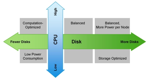
• Compute-intensive workloads will usually be balanced with fewer disks per server.
  • This gives more CPU for a given amount of disk access.
  • You could go down to six or eight disks and get more nodes or more capable CPU’s
• Data-heavy workloads will take advantage of more disks per server.
  • Data-heavy means more data access per query, as opposed to more total data stored.
  • More disks gets more I/O bandwidth regardless of disk size
• Network capacity tends to go up with high-disk density
  • Jobs with a lot of output use higher network bandwidth along with more disk.
    • Output creates three copies of each block; two are across the network.
    • ETL/ELT and sorting are examples of jobs that:
      • Move the entire dataset across the network
      • Have output about the size of the input
• Storage-heavy workloads
  • Have relatively little CPU per stored GB
  • Favor large disks for high capacity and low power consumption per stored GB
  • The benefit is abundant space.
  • The drawback is time and network bandwidth to recover from a hardware failure
• Heterogeneous storage can allow a mix of drives on each machine.
  • Just two archival drives on each node can double the storage capacity of a cluster.
  • Beware the prolonged impact on performance of a disk or node failure.

• Light Processing Configuration (1U/machine): Two hex-core CPUs, 24-64GB memory, and 8 disk drives (1TB or 2TB)
• Balanced Compute Configuration (1U/machine): Two hex-core CPUs, 48-128GB memory, and 12 – 16 disk drives (1TB or 2TB) directly attached using the motherboard controller. These are often available as twins with two motherboards and 24 drives in a single 2U cabinet.
• Storage Heavy Configuration (2U/machine): Two hex-core CPUs, 48-96GB memory, and 16-24 disk drives (2TB – 4TB). This configuration will cause high network traffic in case of multiple node/rack failures.
• Compute Intensive Configuration (2U/machine): Two hex-core CPUs, 64-512GB memory, and 4-8 disk drives (1TB or 2TB)